Gradient descent is one of the most used algorithms to optimize a function. Optimizing a function means finding the hyperparameter values for that function that give us the best possible outcome.
Gradient descent has broad applications, but in this text, we will focus on its use in Machine Learning to minimize model loss in a linear function.
Cost function
Before optimizing anything, we first need a way to measure performance. This is where the loss function comes in. In simple terms, the loss function tells us how far off our model’s predictions are from the actual values. It’s a crucial guide for improving our model.
Some of the most commonly used loss functions include Mean Squared Error (MSE) for regression tasks and cross-entropy for classification problems.
Mean Squared Error
The Mean Squared Error (MSE) is the average of the squared differences between the observed (actual) values and the values predicted by the model. By squaring the differences, we ensure that negative errors don’t cancel out positive ones. You might wonder why we don’t simply take the absolute differences instead. The reason is that squaring the errors penalizes larger mistakes more heavily than smaller ones, which can be useful in emphasizing and correcting significant prediction errors. Mean Squared error is represented by the follwing equation:
![\[\text{MSE} =\frac{1}{n} \sum_{i=1}^{n}(y - \hat y)^2\]](https://sebastiandev.com/wp-content/ql-cache/quicklatex.com-7be925b8d345a944cef879290f89d6f8_l3.png "Rendered by QuickLaTeX.com")
Where  is the predicted value and
  is the observed value./
Illustrative example
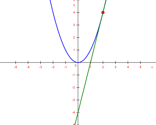
Imagine we have a linear model, represented by a red line, and we want to fit it to a set of data points, shown as black dots. Try to find the best hyperparameters—specifically the slope and the bias—that minimize the model’s error. This error is measured using Mean Squared Error (MSE), which we can visualize as blue squares representing the squared distances between the predicted values on the red line and the actual data points. The smaller these blue squares, the better our model fits the data.
Equation: y = 1.00x + 1.00
MSE: 0
What is the gradient?
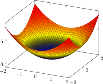
Let’s say we want to optimize a loss function defined by the equation  , where represents the loss value and xxx is the hyperparameter we want to optimize. If we set
  , the loss becomes
While it’s easy to see that the optimal value of  is 0—since we know the shape of the function—in real-world scenarios, the loss function is often much more complex and not visually obvious. So, how can we figure out whether to increase or decrease to reduce the loss?
Spoiler alert: we can do this by calculating the gradient.
By taking the derivative of the loss function with respect to , we obtain the gradient at that point. For , the derivative of  is
is  , so the gradient is
  . This gradient represents the slope of the tangent line at that point.
To minimize the loss, we want to move in the direction that reduces the loss the fastest—that is, in the opposite direction of the gradient. Our goal is to reach a point where the gradient is 0 (or very close to it), which indicates that we’ve found a minimum in the loss function.
Learning rate
However, there are situations where we might start far from the optimal value of our parameter. In such cases, the gradient tends to be steeper—the farther we are from the minimum, the larger the gradient usually is. This suggests that we might want to take larger steps when the gradient is large, and smaller steps when the gradient is small.
This is where the learning rate comes into play. The learning rate is a small positive value that controls how much of the gradient we actually use to update our parameter. Instead of subtracting the full gradient from our parameter, we subtract only a fraction of it. This helps us move in the direction of lower loss without overshooting the minimum.
Gradien descent step by step
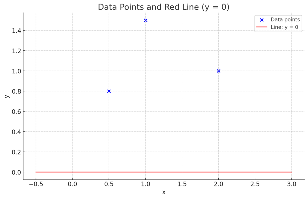
For the following dataset lets build a linear model to make some predictions:
![\[((x_1, y_1) = (0.5, 0.8))\]](https://sebastiandev.com/wp-content/ql-cache/quicklatex.com-0c12ddaf649adb49aaf65f19c5a486a9_l3.png "Rendered by QuickLaTeX.com")
![\[((x_2, y_2) = (2.0, 1.0)\]](https://sebastiandev.com/wp-content/ql-cache/quicklatex.com-982a3b171fefd990d2cec6e45f5f4db2_l3.png "Rendered by QuickLaTeX.com")
![\[((x_3, y_3) = (1.0, 1.5))\]](https://sebastiandev.com/wp-content/ql-cache/quicklatex.com-b86c4068e6c6aca4bbd7a82ba3ecfdef_l3.png "Rendered by QuickLaTeX.com")
In a linear regression model, we have two parameters: the slope and the intercept. Therefore, we need to calculate the gradient for both of them.
![\[f(x) = mx + b\]](https://sebastiandev.com/wp-content/ql-cache/quicklatex.com-3897816ee97d19ea0a7ad540e6d0149f_l3.png "Rendered by QuickLaTeX.com")
Where:
 is the slope,
 is the intercept
Before starting we assking any value both variables to have something to improve on.
Step 1: Initialize paremeters
Before starting the optimization process, we assign an initial value to both variables so we have something to improve upon.


Step 2: Calculate Loss
We’ll use Mean Squared Error (MSE):
![\[\text{Loss}=\frac{1}{n} \sum_{i=1}^{n} (y_i - f(x_i))^2 =\frac{1}{n} \sum_{i=1}^{n} (y_i -(mx_i + b))^2 \]](https://sebastiandev.com/wp-content/ql-cache/quicklatex.com-f526eaecc582fc639e33dfe39bd702ba_l3.png "Rendered by QuickLaTeX.com")
Predictions with 
 for all x values.
Step 3: Compute gradients
We calculate the partial derivatives of the loss with respect to and :
Gradient with respect to :
![\[\frac{\partial \text{Loss}}{\partial m} = -\frac{2}{n} \sum_{i=1}^{n} x_i \left( y_i - (m x_i + b) \right)\]](https://sebastiandev.com/wp-content/ql-cache/quicklatex.com-ca146130d8edb55b3f3ab07415f70821_l3.png "Rendered by QuickLaTeX.com")
![\[\frac{\partial \text{Loss}}{\partial m} = -\frac{2}{3} \left[ 0.5 \cdot (0.8 - 0) + 2 \cdot (1 - 0) + 1 \cdot (1.5 - 0) \right] = -\frac{2}{3} (3.9) = -2.6\]](https://sebastiandev.com/wp-content/ql-cache/quicklatex.com-2aea86bcf0226413eb7bd11f592edf45_l3.png "Rendered by QuickLaTeX.com")
Gradient with respect to :
![\[\frac{\partial \text{Loss }}{\partial b} = -\frac{2}{n} \sum_{i=1}^{n} \left( y_i - (m x_i + b) \right)\]](https://sebastiandev.com/wp-content/ql-cache/quicklatex.com-a49a2fe78682bb930ea1733309af5340_l3.png "Rendered by QuickLaTeX.com")
![\[\frac{\partial \text{Loss}}{\partial m} = -\frac{2}{3} \left[ (0.8 - 0) + (1 - 0) + (1.5 - 0) \right] = -\frac{2}{3} (3.3) = -2.2\]](https://sebastiandev.com/wp-content/ql-cache/quicklatex.com-d7f84fde88f58e970072931408671cfa_l3.png "Rendered by QuickLaTeX.com")
Step 4: Update parameters
Using a learning rate  , we update :
![\[m_{\text{new}} = m_{\text{old}} - \alpha \cdot \frac{\partial \text{Loss}}{\partial m}\]](https://sebastiandev.com/wp-content/ql-cache/quicklatex.com-5b597926206cf698daaa2b070707e418_l3.png "Rendered by QuickLaTeX.com")
![\[m_{\text{new}} = 0 - 0.1 \cdot (-2.6) = 0.26\]](https://sebastiandev.com/wp-content/ql-cache/quicklatex.com-fe5c7cea205f826214b7bfc6b4575833_l3.png "Rendered by QuickLaTeX.com")
Next, we update
![\[m_{\text{new}} = m_{\text{old}} - \alpha \cdot \frac{\partial \text{Loss}}{\partial b}\]](https://sebastiandev.com/wp-content/ql-cache/quicklatex.com-89230328aef4a93b125dbe4cae98573c_l3.png "Rendered by QuickLaTeX.com")
![\[m_{\text{new}} = 0 - 0.1 \cdot (-2.6) = 0.22\]](https://sebastiandev.com/wp-content/ql-cache/quicklatex.com-3a3ed3a6b33c58d9e007ac9b37df6804_l3.png "Rendered by QuickLaTeX.com")
Note: We subtract the gradient from the current value because we want to move in the opposite direction of the gradient, as explained earlier.
Now, we plug these updated values for mmm and bbb into our linear function:
![\[f(x) = 0.26x + 0.22\]](https://sebastiandev.com/wp-content/ql-cache/quicklatex.com-8c1c1ce051e2adb53231de3b6e268d81_l3.png "Rendered by QuickLaTeX.com")
And we plot the updated model:
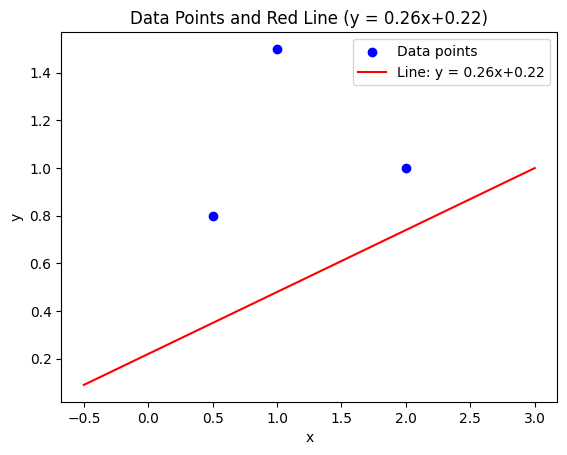
The model has significantly improved compared to the initial version.
After continuing the iterations for 3 more steps, we arrive at the following values:


These values yield the following model:
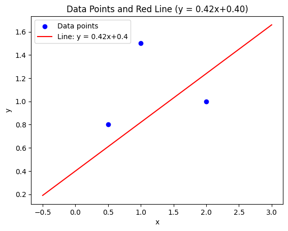
Note: The learning rate α=0.1\alpha = 0.1α=0.1 is not an ideal value. Typically, smaller learning rates are used, as larger values may cause the model to have trouble converging.

 .
. loss) or square the loss (
 loss).

 .
.
