Neural networks are at the core of modern artificial intelligence, powering everything from image recognition and natural language processing to medical diagnostics and self-driving cars. While they may seem complex due to their mathematical foundations, they rely on fundamental calculus concepts that even someone with a high school diploma can understand.
This post explores how neural networks work and how they are trained to recognize patterns in data like text and images—all without using overly technical or confusing lingo.
Neurons
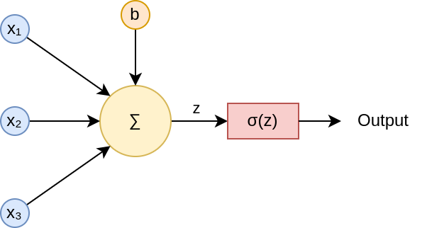
An artificial neuron is the elementary component of a neural network. Neurons receive 1 or more inputs and plug them into a function to produce an output. This function calculates a weighted sum of the inputs and adds a bias term. It does so by multiplying the inputs by their corresponding weight and then adding the bias term.
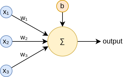
For a neuron with 3 inputs, such as the one in the image, the neuron calculates:  . Where
  is the prediction or output. Very simple.
how do we set the value of our weights and bias (parameters)?
Imagine we want to use our neural network to predict the grade (target) for a course by giving it the hours we studied (input), and we have the following data:
| Hours Studied (input) | Grade (target) |
| 2 | 3 |
| 4 | 5 |
| 6 | 4 |
| 8 | 6 |
| 10 | 8 |
For this scenario, we have one input variable and one target variable. Our neuron’s calculation follows the equation:
![\[\hat y = x_1 w_1 + b\]](https://sebastiandev.com/wp-content/ql-cache/quicklatex.com-edecc209278c5b1c7151db44862b27da_l3.png "Rendered by QuickLaTeX.com")
If this equation looks familiar, that’s because it represents the equation of a line. Our goal is to find the best values for  (slope) and
  (intercept) that allow the model to fit our data optimally.
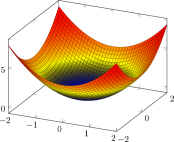
To evaluate how well the model fits, we calculate the Mean Squared Error (MSE)—the average squared distance between each data point and the predicted values from our model. The reason we square the distances is to ensure that negative and positive errors don’t cancel each other out.
To find the best-fitting model, we start with random values for and , then adjust them to minimize the MSE. The values that result in the lowest MSE define the optimal model for our dataset.
Try yourself to find the values that minimize the MSE:
Adjust parameters to Fit Points
Equation: y = 1.00x + 1.00
MSE: 0
For learning purposes, we used a trial-and-error approach to estimate the best values for www and bbb. However, in real neural networks, these parameters are optimized using gradient descent
The most optimum values for this example are  and
and  .
.
Onece model has been optimized, we can use it to predict outcomes for unknown data by plugging the input into our equation. For example, we want to predict our grade if we studied for 7 hours, but we don’t have specific data for this case. Although we don’t have this exact data point in our dataset, our model can generalize based on the learned relationships and give us an approximate grade value.
![\[\hat y = wx+b\]](https://sebastiandev.com/wp-content/ql-cache/quicklatex.com-71ec7a017c1dc2f35c2233ea50ab961e_l3.png "Rendered by QuickLaTeX.com")
![\[ = 0.55x + 1.9\]](https://sebastiandev.com/wp-content/ql-cache/quicklatex.com-8bff856bf5f51b11c2d6081d628f7aa7_l3.png "Rendered by QuickLaTeX.com")
![\[= 0.55(7)+1.9 = 5.75\]](https://sebastiandev.com/wp-content/ql-cache/quicklatex.com-30415b27bb4aa2ff029064e0b3b04e7d_l3.png "Rendered by QuickLaTeX.com")
New Graph of the Line, Evaluated Point, and Given Points
According to our model, if we study 7 hours, we are expected to get a grade of 5.75.
Note. This example has only one input, but the process is the same if you have more than one input.
Neural Networks
Now that we know how a neuron works, we can stack them in layers, connecting all neurons in one layer to all the neurons in the previous layer. This kind of neural network is called a fully connected neural networks, and they look like this:
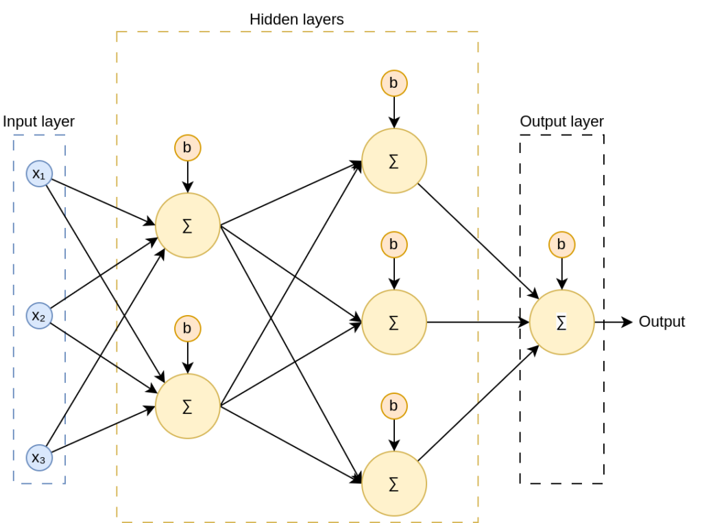
Observe how, for the hidden neurons (those in the hidden layers), the outputs from the preceding layers serve as inputs. Also, note that although weights are not represented in the image, all connections have their own weight.
By stacking neurons, the network can model not just linearly shaped data but also data with complex patterns and structures. Think of each neuron as a line, and by stacking multiple lines, you can build a model that can make generalizations (predictions) from your data.
Activation function
So far, we have sum a bunch of lines, but there is a problem with that; The sum of two or more lines is a line. So, a neural network like the one in the image above would give us a single line as an output. Therefore, it wouldn’t be any better than a single neuron.
We must apply some nonlinearity to each neuron to prevent neural networks from collapsing into a single neuron. This nonlinearity we use is called activation function, and are denoted as  . Where
  .
.
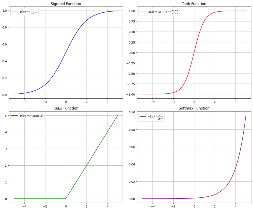
Some of the most known activation functions are:
- Softmax
- Sigmoid
- RELU
- Tanh
![\[\sigma(z_i)=\frac{e^x_i}{\sum{e^x_j}}\]](https://sebastiandev.com/wp-content/ql-cache/quicklatex.com-abe72f52cbec5e88e76d9d86d6234053_l3.png "Rendered by QuickLaTeX.com")
![\[\sigma(z)=\frac{1}{1+e^{-z}}\]](https://sebastiandev.com/wp-content/ql-cache/quicklatex.com-b87875edbe9e31ada0e6da720012be54_l3.png "Rendered by QuickLaTeX.com")
![\[\sigma(z)=max(0, x)\]](https://sebastiandev.com/wp-content/ql-cache/quicklatex.com-e9732987c8672a142134ccb2d8108964_l3.png "Rendered by QuickLaTeX.com")
![\[\sigma(z)=tanh(z)=\frac{e^x - e^{-x}}{e^x + e^{-x}}\]](https://sebastiandev.com/wp-content/ql-cache/quicklatex.com-6ddb3193a352bf43031787fa6d367b61_l3.png "Rendered by QuickLaTeX.com")
Don’t worry if you don’t understand these equations; just focus on the fact that these activation functions add nonlinearity, and they look like this:
We applied an activation function to the outputs of each neuron, enabling us to process these outputs without collapsing and to fit data that was non-linearly shaped or followed complex patterns. The prediction for the neuron
The resulting diagram of a neuron including the activation function would be:
Backpropagation
When we run the calculations through our neural network for the first time, we’ll get a random output since all the weights and biases (parameters) are initialized randomly.
To optimize these parameters, we need to calculate the error for the obtained output and then propagate that error backward through all the previous layers.
Then, we use the gradient descent to optimize the parameters across the network. Neurons that contribute the most to the error will be penalized, and their impact will be reduced by adjusting their weights. On the other hand, neurons that contribute more to the desired output will gain more importance, as their weights are adjusted to improve the overall network performance.
If you’re interested in learning how backpropagation works and the math behind it, you can read my post about backpropagation.
Now what?
To sum up, training a neural network involves iterating through numerous steps of forward and backward passes and adjusting the weights and biases at each layer to minimize the error. This is achieved through techniques like gradient descent and backpropagation, which penalize neurons responsible for the most significant errors. At the same time, those that contribute positively to the output are strengthened. Over time, this process allows the network to learn from the data and make increasingly accurate predictions.
Now that we understand how neural networks work and how backpropagation and gradient descent are used to optimize their parameters, we can apply these networks to process a wide range of data. For instance, in image processing, each pixel can serve as an input to the network, while in Natural Language Processing (NLP), words or even characters can be the inputs. This versatility allows neural networks to solve complex problems across various domains, making them invaluable in fields like computer vision, NLP, and beyond.
![\[\text{MSE} =\frac{1}{n} \sum_{i=1}^{n}(y - \hat y)^2\]](https://sebastiandev.com/wp-content/ql-cache/quicklatex.com-7be925b8d345a944cef879290f89d6f8_l3.png "Rendered by QuickLaTeX.com")
 is the observed value./
 , where
  , the loss becomes
 is 0—since we know the shape of the function—in real-world scenarios, the loss function is often much more complex and not visually obvious. So, how can we figure out whether to increase or decrease
  is
is  , so the gradient is
  . This gradient represents the slope of the tangent line at that point.
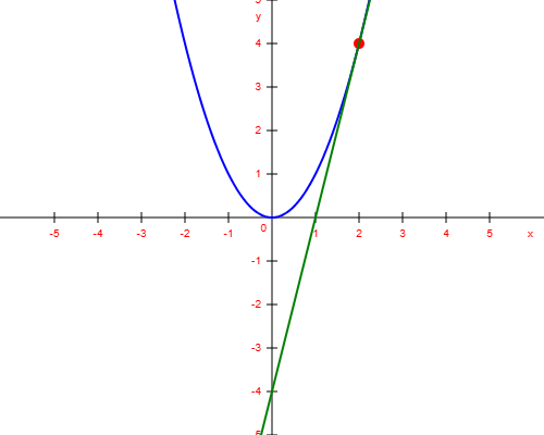
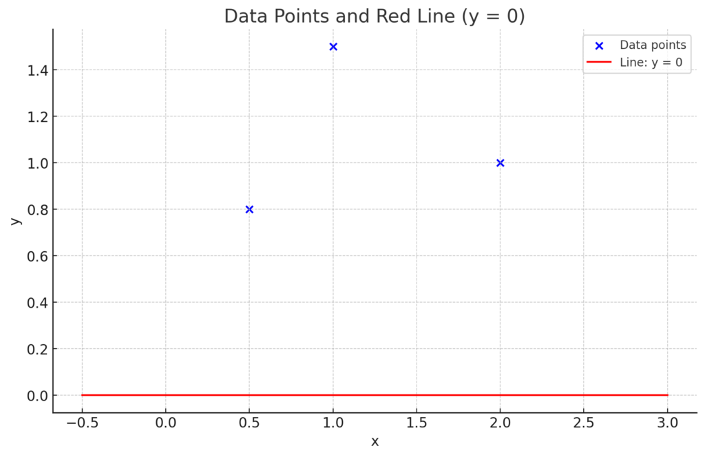
![\[((x_1, y_1) = (0.5, 0.8))\]](https://sebastiandev.com/wp-content/ql-cache/quicklatex.com-0c12ddaf649adb49aaf65f19c5a486a9_l3.png "Rendered by QuickLaTeX.com")
![\[((x_2, y_2) = (2.0, 1.0)\]](https://sebastiandev.com/wp-content/ql-cache/quicklatex.com-982a3b171fefd990d2cec6e45f5f4db2_l3.png "Rendered by QuickLaTeX.com")
![\[((x_3, y_3) = (1.0, 1.5))\]](https://sebastiandev.com/wp-content/ql-cache/quicklatex.com-b86c4068e6c6aca4bbd7a82ba3ecfdef_l3.png "Rendered by QuickLaTeX.com")
![\[f(x) = mx + b\]](https://sebastiandev.com/wp-content/ql-cache/quicklatex.com-3897816ee97d19ea0a7ad540e6d0149f_l3.png "Rendered by QuickLaTeX.com")
 is the slope,

![\[\text{Loss}=\frac{1}{n} \sum_{i=1}^{n} (y_i - f(x_i))^2 =\frac{1}{n} \sum_{i=1}^{n} (y_i -(mx_i + b))^2 \]](https://sebastiandev.com/wp-content/ql-cache/quicklatex.com-f526eaecc582fc639e33dfe39bd702ba_l3.png "Rendered by QuickLaTeX.com")

 for all x values.
![\[\frac{\partial \text{Loss}}{\partial m} = -\frac{2}{n} \sum_{i=1}^{n} x_i \left( y_i - (m x_i + b) \right)\]](https://sebastiandev.com/wp-content/ql-cache/quicklatex.com-ca146130d8edb55b3f3ab07415f70821_l3.png "Rendered by QuickLaTeX.com")
![\[\frac{\partial \text{Loss}}{\partial m} = -\frac{2}{3} \left[ 0.5 \cdot (0.8 - 0) + 2 \cdot (1 - 0) + 1 \cdot (1.5 - 0) \right] = -\frac{2}{3} (3.9) = -2.6\]](https://sebastiandev.com/wp-content/ql-cache/quicklatex.com-2aea86bcf0226413eb7bd11f592edf45_l3.png "Rendered by QuickLaTeX.com")
![\[\frac{\partial \text{Loss }}{\partial b} = -\frac{2}{n} \sum_{i=1}^{n} \left( y_i - (m x_i + b) \right)\]](https://sebastiandev.com/wp-content/ql-cache/quicklatex.com-a49a2fe78682bb930ea1733309af5340_l3.png "Rendered by QuickLaTeX.com")
![\[\frac{\partial \text{Loss}}{\partial m} = -\frac{2}{3} \left[ (0.8 - 0) + (1 - 0) + (1.5 - 0) \right] = -\frac{2}{3} (3.3) = -2.2\]](https://sebastiandev.com/wp-content/ql-cache/quicklatex.com-d7f84fde88f58e970072931408671cfa_l3.png "Rendered by QuickLaTeX.com")
 , we update
 ![\[m_{\text{new}} = m_{\text{old}} - \alpha \cdot \frac{\partial \text{Loss}}{\partial m}\]](https://sebastiandev.com/wp-content/ql-cache/quicklatex.com-5b597926206cf698daaa2b070707e418_l3.png "Rendered by QuickLaTeX.com")
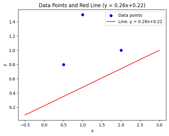
![\[m_{\text{new}} = 0 - 0.1 \cdot (-2.6) = 0.26\]](https://sebastiandev.com/wp-content/ql-cache/quicklatex.com-fe5c7cea205f826214b7bfc6b4575833_l3.png "Rendered by QuickLaTeX.com")
![\[m_{\text{new}} = m_{\text{old}} - \alpha \cdot \frac{\partial \text{Loss}}{\partial b}\]](https://sebastiandev.com/wp-content/ql-cache/quicklatex.com-89230328aef4a93b125dbe4cae98573c_l3.png "Rendered by QuickLaTeX.com")
![\[m_{\text{new}} = 0 - 0.1 \cdot (-2.6) = 0.22\]](https://sebastiandev.com/wp-content/ql-cache/quicklatex.com-3a3ed3a6b33c58d9e007ac9b37df6804_l3.png "Rendered by QuickLaTeX.com")
![\[f(x) = 0.26x + 0.22\]](https://sebastiandev.com/wp-content/ql-cache/quicklatex.com-8c1c1ce051e2adb53231de3b6e268d81_l3.png "Rendered by QuickLaTeX.com")


![\[L= \sum (\hat{y}- y)^2\]](https://sebastiandev.com/wp-content/ql-cache/quicklatex.com-25ed125b76f5aaeae3a96b1be46c25c1_l3.png "Rendered by QuickLaTeX.com")
![\[L=(2-9)^2=49\]](https://sebastiandev.com/wp-content/ql-cache/quicklatex.com-a407f85b9aeb48a006889b2fd93705cc_l3.png "Rendered by QuickLaTeX.com")
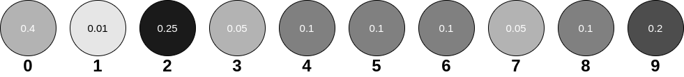
![\[L=P(y)\]](https://sebastiandev.com/wp-content/ql-cache/quicklatex.com-09786419d5c9f2e113e09afa890d70f7_l3.png "Rendered by QuickLaTeX.com")
![\[L=P(9)=0.2\]](https://sebastiandev.com/wp-content/ql-cache/quicklatex.com-03afdbbf294e3a3b6c59c8b2bc7bf5cc_l3.png "Rendered by QuickLaTeX.com")
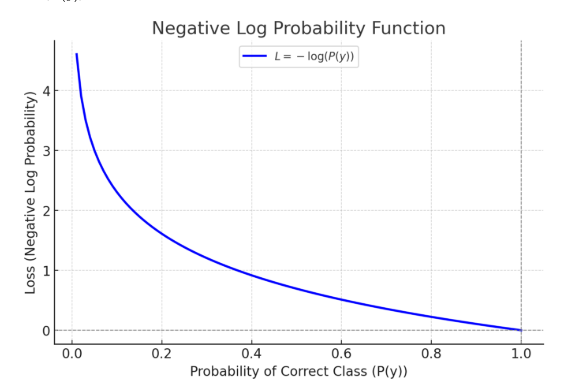
![\[L=-\log P(y)\]](https://sebastiandev.com/wp-content/ql-cache/quicklatex.com-261d417bd1498af29d4aa3596b264399_l3.png "Rendered by QuickLaTeX.com")
![\[L = -\log P(9) = -\log (0.2) = 0.70\]](https://sebastiandev.com/wp-content/ql-cache/quicklatex.com-19576dcb5f3c66d00dbd5aba6acb6c34_l3.png "Rendered by QuickLaTeX.com")
![\[L = -\log P(9) = -\log (0.95) = 0.02\]](https://sebastiandev.com/wp-content/ql-cache/quicklatex.com-5fd8c0d8b12074134e77f7dcf0ae86f5_l3.png "Rendered by QuickLaTeX.com")

 .
. loss) or square the loss (
 loss).

 .
.